 Equilibria and the Phase Line
 Equilibria and the Phase Line

Solving a differential equation can be done in three major ways: analytical, qualitative, and numerical. We have seen some examples of differential equations solved through analytical techniques (for example: linear, separable, and Bernoulli equations). Euler's Method (though very primitive) illustrates the use of numerical techniques in solving differential equations. For the qualitative approach, we have defined the slope field of a differential equation and showed how this can be helpful when other techniques fail.
When the differential equation is autonomous, more can be said
about the solutions using qualitative techniques.
Consider the autonomous differential equation
![]()
where f(y) is a function. Clearly we recognize a separable equation. So we know how to solve it via the analytical technique. First we look for the constant solutions as the roots of the equation
![]()
Then to find the nonconstant solutions we separate the variable
![]()
and integrate
![]()
Note that the integration may be hard if not impossible to carry out. So it may not be possible to use the analytical technique.
In this case, one may try numerical techniques. Unfortunately, numerical techniques fail if f(y) contains a parameter and we need to make conclusions relative to this parameter. For example, recall the logistic equation with harvesting (with a constant rate H)
![]()
where y(t) is the population of the given species at time t. In
order to find the optimal rate H (which makes hunters happy as well
as ecologists worried about preserving the species), numerical
techniques may not be the best tool to use. Here we will see how new
ideas based on a graphical approach will help us to say something about the
solutions. Be aware that these ideas are only valid for
autonomous equations.
Equilibria of Autonomous Equations
Consider the autonomous equation
![]()
The equilibria or constant solutions of this differential equation are the roots of the equation
![]()
Using the existence and uniqueness theorem, these constant solutions
will cut the entire plane (where the solutions live) into independent
regions. This means, if an initial condition belongs to one of the
regions, then the solution satisfying the initial condition will stay
in that region all the time.
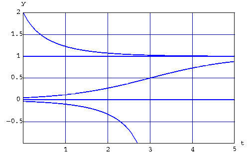
Example. Consider the logistic equation
![]()
Its equilibria are y=0 and y=1. Consider the solution y(t) to the IVP
![]()
Since 0 <y(0) < 1, then we must have
![]()
In the next picture, we draw few solutions associated to initial
conditions in the different regions (0 < y < 1, y < 0, and 1 <
y)
|
Note that in this example, any solution y(t) is increasing if 0 < y(0) < 1 is satisfied. So one may wonder whether a similar conclusion is true in general. Consider again the autonomous equation
![]()
Assume that ![]() and
and ![]() (
( ![]() ) are equilibria (that is
) are equilibria (that is ![]() and
and
![]() ).
Assume moreover that f(y) has a constant sign on the
interval
).
Assume moreover that f(y) has a constant sign on the
interval ![]() .
Assume that f(y) is positive and consider the
solution to the IVP
.
Assume that f(y) is positive and consider the
solution to the IVP
![]()
where ![]() . We know that we will have
. We know that we will have ![]() for every t. Since
for every t. Since
![]()
we must have  for all t. This
clearly implies that y(t) is always increasing. So the sign of
f(y) helps us determine the behavior of the solutions (whether they are
increasing or decreasing).
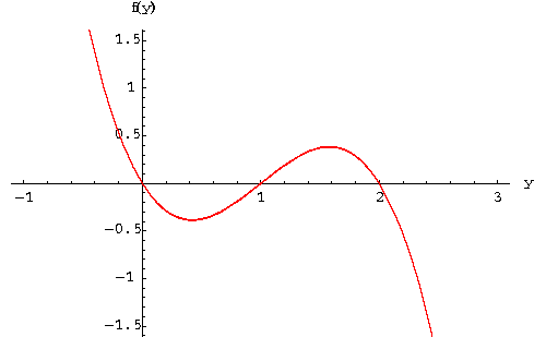
Example. Consider the autonomous equation
![]()
where the graph of f(y) is given below
|
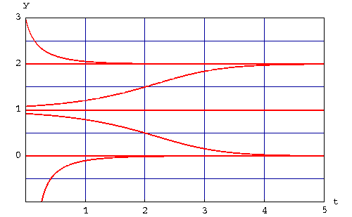
From the graph, we can determine the equilibria. They are y=0, y=1, and y=2. Using the discussion above, we obtain the following information:
|
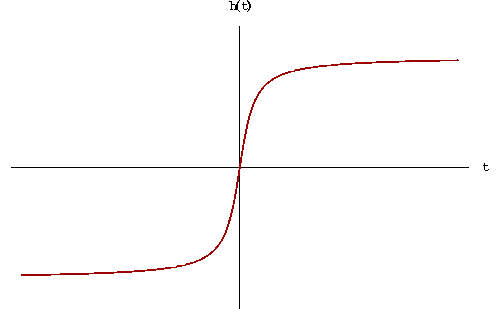
Remark. Recall that if the function h(t) is increasing or decreasing, then the following hold :
![]()
![]()
![]()
The next image illustrates this conclusion better than words can do.
|
Example. Consider the solution to the initial value problem
![]()
where the graph of f(y) is given below
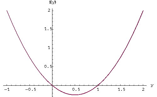
|
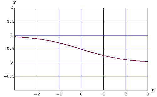
Discuss the limit of y(t) when ![]() .
.
Answer. Using the above results, we know that for the given initial condition, y(t) is decreasing and for every t we have
![]()
The above remark implies that ![]() exist and we have
exist and we have
![]()
Since y(t) is not a constant solution (because y(0)=0.5), then we have
![]()
On the other hand, since
![]()
and y is solution to the autonomous equation y'=f(y), then the only possibilities for both limits are the equilibria 0,1, and 2. Clearly if we put everything together, we conclude that
![]()
|
Summary. Let us write down some general steps to follow when dealing with the autonomous equation
![]()
![]()
Draw the constant solutions. Note that here we are drawing y versus t.
Remark. You must be very careful here, since two graphs will be
drawn: one for the function f(y) (versus y) and another one for
the solutions, where this time y is on the vertical axis while t is
on the horizontal axis. Keep in mind that the second graph is the
most important one, since it deals with what we are looking for: the
solutions of the differential equation.
Example. Draw some solutions for the equation
![]()
Answer. Note that this equation models the logistic growth with threshold. The equilibria or constant solutions are given by
![]()
or y=0, y=2, and y=5. The graph of the function f(y) =
.2y(5-y)(y-2) is given in the next picture
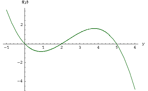
|
So we have:
![]()
![]()
![]()
![]()
In the picture below we draw some solutions
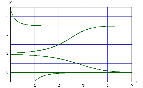
|
Phase Line
Let us reconsider the above example. Let us focus our attention on the solutions
which satisfy the initial condition ![]() and
and ![]() .
We already know that
.
We already know that
![]()
It is somehow amazing that this conclusion is valid regardless whether
![]() is close
to 5 or close to 2. In this case we say that the
equilibrium point 5 is attractive from below. In fact, in this
example, this equilibrium point is attractive from below and above.
On the other hand, the solutions get away from the equilibrium point 2
from below and above. We will say that the equilibrium point 2 is
repelling. Note that there is no general agreement on the words used to describe these phenomena.
is close
to 5 or close to 2. In this case we say that the
equilibrium point 5 is attractive from below. In fact, in this
example, this equilibrium point is attractive from below and above.
On the other hand, the solutions get away from the equilibrium point 2
from below and above. We will say that the equilibrium point 2 is
repelling. Note that there is no general agreement on the words used to describe these phenomena.
Definition. Classification of Equilibrium
Points.
Consider the autonomous equation
![]()
Assume that ![]() is an equilibrium point (that is
is an equilibrium point (that is ![]() ).
).
![]()
Example. Classify the equilibrium points of the equation
![]()
as source, sink, or node.
Answer. The equilibrium points are 0, 2, and 5. Using the above
results, we see that 0 and 5 are sinks while 2 is a source.
Example. Find and classify the equilibrium points of the equation
![]()
as source, sink, or node.
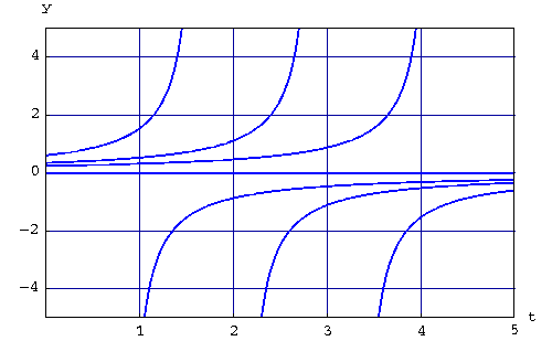
Answer. It is easy to see that the only equilibrium point is 0.
Since ![]() is always positive, then the solutions will always
be increasing. Using previous results, we conclude:
is always positive, then the solutions will always
be increasing. Using previous results, we conclude:
![]()
![]()
|
There is a very nice way to put all this information together. Indeed, draw a vertical line (where the variable describing it is y) and start by marking the equilibrium points of the equation
![]()
on the y-axis.
Then using the sign of f(y), we draw arrows pointing upward in a region
where f(y) is positive, and downward in a region where f(y) is
negative. This vertical line is called the phase line of the
equation.
An equilibrium point is a sink, if the arrows on both sides point towards the equilibrium point, and it is a source, if both arrows point away from it.
Example. Draw the phase line of the equations
![]()
and
![]()
Answer. We will use our previous knowledge to get the two phase
lines

|
and

|
You can readily see, that an equilibrium point is a sink, if the arrows on both sides point towards the equilibrium point, and that it is a source, if both arrows point away from it.

 S.O.S. MATHematics home page
 Do you need more help? Please post your question on our S.O.S. Mathematics CyberBoard.

Author: Mohamed Amine Khamsi